Clase 20: Regresiones
En esta clase revisaremos los conceptos econométricos de Mínimos Cuadrados Ordinarios (OLS por sus siglas en inglés) y Modelo Autorregresivo (AR por sus siglas en inglés).
Para esto vamos a utilizar la librería statsmodels: https://www.statsmodels.org/stable/install.html
Mínimos Cuadrados Ordinarios (Ordinary Least Squares)
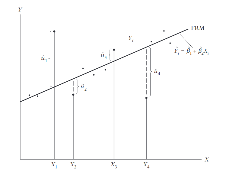
Buscamos estimar la Función de Regresión Poblacional (FRP), sin embargo esta no es observable directamente. Para esto vamos a utilizar una estimación que llamaremos la Función de Regresión Muestral (FRM):
FRP: \(Y_i = \beta_1 + \beta_2 X_i + \mu_i\)
FRM: \(Y_i = \hat{\beta}_1 + \hat{\beta}_2 X_i + \hat{\mu}_i = \hat{Y}_i - \hat{\mu}_i\), donde \(\hat{Y}_i\) es el valor estimado (media condicional) de \(Y_i\).
Entonces, en OLS vamos a minimizar el error \(\hat{\mu}_i = Y_i - \hat{Y_i}\) $\(\begin{align} \sum u_i^2 &= \sum (Y_i-\hat{Y}_i)^2 \\ &= \sum (Y_i - \hat{\beta}_1 - \hat{\beta}_2 X_i)^2 \end{align}\)$
from IPython.display import Image
Image("OLS1.png")
import pandas as pd
import numpy as np
df = pd.read_stata("/home/felix/Dropbox/Computational_Economics/Intro_python/Data_OLS_AR/Casen2020.dta");
/home/felix/miniconda3/lib/python3.9/site-packages/pandas/io/stata.py:1417: UnicodeWarning:
One or more strings in the dta file could not be decoded using utf-8, and
so the fallback encoding of latin-1 is being used.  This can happen when a file
has been incorrectly encoded by Stata or some other software. You should verify
the string values returned are correct.
  warnings.warn(msg, UnicodeWarning)
detalle_ingreso = df.ytrabajocor.describe()
detalle_ingreso
count    7.350900e+04
mean     5.783447e+05
std      1.264676e+06
min      4.000000e+00
25%      2.000000e+05
50%      3.681670e+05
75%      6.500000e+05
max      2.250000e+08
Name: ytrabajocor, dtype: float64
df2 = df[(df.ytrabajocor>0) & (df.ytrabajocor<10_000_000) & (df.ytrabajocor.notna())]
df2.ytrabajocor.describe()
count    7.345000e+04
mean     5.617230e+05
std      6.973099e+05
min      4.000000e+00
25%      2.000000e+05
50%      3.674275e+05
75%      6.500000e+05
max      9.850000e+06
Name: ytrabajocor, dtype: float64
plt.plot(df2.ytrabajocor, 'g')
plt.xlabel("Observación")
plt.ylabel('Ingreso del trabajo')
---------------------------------------------------------------------------
NameError                                 Traceback (most recent call last)
<ipython-input-5-b7adf0787577> in <module>
----> 1 plt.plot(df2.ytrabajocor, 'g')
      2 plt.xlabel("Observación")
      3 plt.ylabel('Ingreso del trabajo')

NameError: name 'plt' is not defined
import matplotlib.pyplot as plt
fig = plt.figure(figsize=(8, 8))
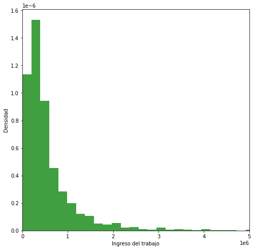
plt.hist(df2.ytrabajocor, 50, density=True, facecolor='g', alpha=0.75)
plt.xlim([0, 5_000_000])
plt.xlabel('Ingreso del trabajo')
plt.ylabel('Densidad')
plt.show()
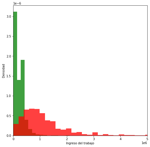
y_educ_bas = df2[["ytrabajocor", "educ"]][df2.educ=="Básica incompleta"].ytrabajocor
y_educ_uni = df2[["ytrabajocor", "educ"]][df2.educ=="Profesional completo"].ytrabajocor
fig = plt.figure(figsize=(8, 8))
plt.hist(y_educ_bas, 50, density=True, facecolor='g', alpha=0.75)
plt.hist(y_educ_uni, 50, density=True, facecolor='r', alpha=0.75)
plt.xlim([0, 5_000_000])
plt.xlabel('Ingreso del trabajo')
plt.ylabel('Densidad')
plt.show()
Datos para la regresión
y = df2.ytrabajocor
X = df2.esc
X = sm.add_constant(X)
X.head()
| const | esc | |
|---|---|---|
| 0 | 1.0 | 12.0 |
| 3 | 1.0 | 15.0 |
| 4 | 1.0 | NaN |
| 5 | 1.0 | 16.0 |
| 7 | 1.0 | 15.0 |
#Hay que limpiar los NaN en variable exógena
df3 = df[(df.ytrabajocor>0) & (df.ytrabajocor<10_000_000) & (df.ytrabajocor.notna()) & (df.esc.notna())]
y = df3.ytrabajocor
X = df3.esc
X = sm.add_constant(X)
X.head()
| const | esc | |
|---|---|---|
| 0 | 1.0 | 12.0 |
| 3 | 1.0 | 15.0 |
| 5 | 1.0 | 16.0 |
| 7 | 1.0 | 15.0 |
| 11 | 1.0 | 14.0 |
y = df3.ytrabajocor
X = df3.esc
X = sm.add_constant(X)
X.head()
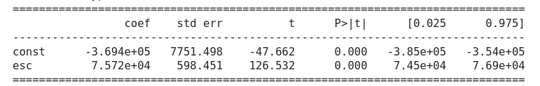
import statsmodels.api as sm
model = sm.OLS(y, X)
results = model.fit()
print(results.summary())
                            OLS Regression Results
==============================================================================
Dep. Variable:            ytrabajocor   R-squared:                       0.183
Model:                            OLS   Adj. R-squared:                  0.183
Method:                 Least Squares   F-statistic:                 1.601e+04
Date:                Mon, 26 Jul 2021   Prob (F-statistic):               0.00
Time:                        22:21:34   Log-Likelihood:            -1.0554e+06
No. Observations:               71466   AIC:                         2.111e+06
Df Residuals:                   71464   BIC:                         2.111e+06
Df Model:                           1
Covariance Type:            nonrobust
==============================================================================
                 coef    std err          t      P>|t|      [0.025      0.975]
------------------------------------------------------------------------------
const      -3.694e+05   7751.498    -47.662      0.000   -3.85e+05   -3.54e+05
esc         7.572e+04    598.451    126.532      0.000    7.45e+04    7.69e+04
==============================================================================
Omnibus:                    64620.243   Durbin-Watson:                   1.630
Prob(Omnibus):                  0.000   Jarque-Bera (JB):          3238679.663
Skew:                           4.257   Prob(JB):                         0.00
Kurtosis:                      34.861   Cond. No.                         43.0
==============================================================================

Notes:
[1] Standard Errors assume that the covariance matrix of the errors is correctly specified.
No. Observations: número de observaciones ocupadas en la regresión.
R-squared: El \(R^2\) es la proporción de la varianza en la variable dependiente que puede ser predicha por las variables independientes. En este caso un 18% de la varianza es explicada por las variables independientes.
Adj R-squared (\(R^2\) ajustado): el \(R^2\) se ajusta para penalizar que se agreguen regresores extraños.
F-statistic (F(Z,)): Es la razón entre el error cuadrático medio del modelo y el error cuadrático medio de los residuos. Nos sirve para determinar la importancia general del modelo.
Criterios de información (AIC y BIC): nos sirven para ver el trade-off entre complejidad del modelo y bondad de ajuste de este.
Image("OLS3.png")
En las filas están las variables con las que regresionamos: constante y educación. En las columnas tenemos:
El coeficiente de las variables independientes y la constante. Acá estamos estimando los \(\beta_i\): \(Y_i = \hat{\beta}_1 + \hat{\beta}_2 X_i + \hat{\mu}_i\)
std err: error estándar asociado a los coeficientes.
t: estadístico t usado para testear la significancia de los coeficientes.
\(P>|t|\): p-value de dos colas usado para testear hipótesis nula de que el coeficiente es cero (\(\alpha=0.05\)).
[0.025 - 0.975]: intervalo de confianza de coeficiente con \(\alpha=0.05\).
#df.loc[df['column name'] condition, 'new column name'] = 'value if condition is met'

df3.loc[df3.sexo=="Hombre", "sexo2"] = 0
df3.loc[df3.sexo=="Mujer", "sexo2"] = 1
/home/felix/miniconda3/lib/python3.9/site-packages/pandas/core/indexing.py:1599: SettingWithCopyWarning:
A value is trying to be set on a copy of a slice from a DataFrame.
Try using .loc[row_indexer,col_indexer] = value instead

See the caveats in the documentation: https://pandas.pydata.org/pandas-docs/stable/user_guide/indexing.html#returning-a-view-versus-a-copy
  self.obj[key] = infer_fill_value(value)
/home/felix/miniconda3/lib/python3.9/site-packages/pandas/core/indexing.py:1720: SettingWithCopyWarning:
A value is trying to be set on a copy of a slice from a DataFrame.
Try using .loc[row_indexer,col_indexer] = value instead

See the caveats in the documentation: https://pandas.pydata.org/pandas-docs/stable/user_guide/indexing.html#returning-a-view-versus-a-copy
  self._setitem_single_column(loc, value, pi)
y = df3.ytrabajocor
X = df3[["esc", "edad", "sexo2"]]
X = sm.add_constant(X)
X.head()
| const | esc | edad | sexo2 | esc2 | |
|---|---|---|---|---|---|
| 0 | 1.0 | 12.0 | 34 | 1.0 | 144.0 |
| 3 | 1.0 | 15.0 | 45 | 0.0 | 225.0 |
| 5 | 1.0 | 16.0 | 57 | 0.0 | 256.0 |
| 7 | 1.0 | 15.0 | 56 | 1.0 | 225.0 |
| 11 | 1.0 | 14.0 | 54 | 1.0 | 196.0 |
df3['exp'] = df3.edad-df3.esc
df3['exp2'] = df3.exp**2
df3['exp_sexo'] = df3.exp*df3.sexo2
y = np.log(df3.ytrabajocor)
X = df3[["esc", "exp", "exp2", "sexo2", "exp_sexo"]]
X = sm.add_constant(X)
X.head()
<ipython-input-18-79fecfcd28f3>:1: SettingWithCopyWarning:
A value is trying to be set on a copy of a slice from a DataFrame.
Try using .loc[row_indexer,col_indexer] = value instead

See the caveats in the documentation: https://pandas.pydata.org/pandas-docs/stable/user_guide/indexing.html#returning-a-view-versus-a-copy
  df3['exp'] = df3.edad-df3.esc
<ipython-input-18-79fecfcd28f3>:2: SettingWithCopyWarning:
A value is trying to be set on a copy of a slice from a DataFrame.
Try using .loc[row_indexer,col_indexer] = value instead

See the caveats in the documentation: https://pandas.pydata.org/pandas-docs/stable/user_guide/indexing.html#returning-a-view-versus-a-copy
  df3['exp2'] = df3.exp**2
<ipython-input-18-79fecfcd28f3>:3: SettingWithCopyWarning:
A value is trying to be set on a copy of a slice from a DataFrame.
Try using .loc[row_indexer,col_indexer] = value instead

See the caveats in the documentation: https://pandas.pydata.org/pandas-docs/stable/user_guide/indexing.html#returning-a-view-versus-a-copy
  df3['exp_sexo'] = df3.exp*df3.sexo2
| const | esc | exp | exp2 | sexo2 | exp_sexo | |
|---|---|---|---|---|---|---|
| 0 | 1.0 | 12.0 | 22.0 | 484.0 | 1.0 | 22.0 |
| 3 | 1.0 | 15.0 | 30.0 | 900.0 | 0.0 | 0.0 |
| 5 | 1.0 | 16.0 | 41.0 | 1681.0 | 0.0 | 0.0 |
| 7 | 1.0 | 15.0 | 41.0 | 1681.0 | 1.0 | 41.0 |
| 11 | 1.0 | 14.0 | 40.0 | 1600.0 | 1.0 | 40.0 |
model = sm.OLS(y, X)
results = model.fit()
print(results.summary())
                            OLS Regression Results
==============================================================================
Dep. Variable:            ytrabajocor   R-squared:                       0.265
Model:                            OLS   Adj. R-squared:                  0.265
Method:                 Least Squares   F-statistic:                     5151.
Date:                Tue, 26 Oct 2021   Prob (F-statistic):               0.00
Time:                        11:08:12   Log-Likelihood:            -1.1887e+05
No. Observations:               71466   AIC:                         2.378e+05
Df Residuals:                   71460   BIC:                         2.378e+05
Df Model:                           5
Covariance Type:            nonrobust
==============================================================================
                 coef    std err          t      P>|t|      [0.025      0.975]
------------------------------------------------------------------------------
const          9.7314      0.030    326.486      0.000       9.673       9.790
esc            0.1522      0.002    100.943      0.000       0.149       0.155
exp            0.0820      0.001     71.234      0.000       0.080       0.084
exp2          -0.0011   1.56e-05    -68.238      0.000      -0.001      -0.001
sexo2         -0.1503      0.021     -7.152      0.000      -0.191      -0.109
exp_sexo      -0.0136      0.001    -23.036      0.000      -0.015      -0.012
==============================================================================
Omnibus:                    31679.342   Durbin-Watson:                   1.650
Prob(Omnibus):                  0.000   Jarque-Bera (JB):           197590.127
Skew:                          -2.052   Prob(JB):                         0.00
Kurtosis:                      10.037   Cond. No.                     1.12e+04
==============================================================================

Notes:
[1] Standard Errors assume that the covariance matrix of the errors is correctly specified.
[2] The condition number is large, 1.12e+04. This might indicate that there are
strong multicollinearity or other numerical problems.
y = np.log(df3.ytrabajocor)
X = df3[["esc", "edad", "sexo2"]]
X = sm.add_constant(X)
X.head()
| const | esc | edad | sexo2 | |
|---|---|---|---|---|
| 0 | 1.0 | 12.0 | 34 | 1.0 |
| 3 | 1.0 | 15.0 | 45 | 0.0 |
| 5 | 1.0 | 16.0 | 57 | 0.0 |
| 7 | 1.0 | 15.0 | 56 | 1.0 |
| 11 | 1.0 | 14.0 | 54 | 1.0 |
model = sm.OLS(y, X)
results = model.fit()
print(results.summary())
                            OLS Regression Results
==============================================================================
Dep. Variable:            ytrabajocor   R-squared:                       0.212
Model:                            OLS   Adj. R-squared:                  0.212
Method:                 Least Squares   F-statistic:                     6423.
Date:                Mon, 26 Jul 2021   Prob (F-statistic):               0.00
Time:                        23:38:58   Log-Likelihood:            -1.2134e+05
No. Observations:               71466   AIC:                         2.427e+05
Df Residuals:                   71462   BIC:                         2.427e+05
Df Model:                           3
Covariance Type:            nonrobust
==============================================================================
                 coef    std err          t      P>|t|      [0.025      0.975]
------------------------------------------------------------------------------
const         10.5982      0.028    380.688      0.000      10.544      10.653
esc            0.1696      0.001    124.958      0.000       0.167       0.172
edad           0.0039      0.000     10.597      0.000       0.003       0.005
sexo2         -0.5787      0.010    -58.179      0.000      -0.598      -0.559
==============================================================================
Omnibus:                    32963.117   Durbin-Watson:                   1.642
Prob(Omnibus):                  0.000   Jarque-Bera (JB):           198868.520
Skew:                          -2.170   Prob(JB):                         0.00
Kurtosis:                       9.925   Cond. No.                         269.
==============================================================================

Notes:
[1] Standard Errors assume that the covariance matrix of the errors is correctly specified.
print('Parámetros: ', results.params)
print('Error estandar: ', results.bse)
print('Valores predichos: ', results.predict())
Parámetros:  const    10.598153
esc       0.169602
edad      0.003898
sexo2    -0.578690
dtype: float64
Error estandar:  const    0.027839
esc      0.001357
edad     0.000368
sexo2    0.009947
dtype: float64
Valores predichos:  [12.18721169 13.31758263 13.5339568  ... 12.31583427 10.77744552
 11.22416493]
Comparar resultados predichos
from statsmodels.sandbox.regression.predstd import wls_prediction_std
prstd, iv_l, iv_u = wls_prediction_std(results)
fig, ax = plt.subplots(figsize=(8,6))
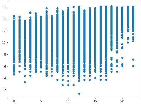
ax.plot(X.esc, y, 'o', label="data")
[<matplotlib.lines.Line2D at 0x7f4486a0d9d0>]
Para ver ejemplos de gráficos en modelos de regresión pueden utilizar https://www.statsmodels.org/stable/examples/notebooks/generated/regression_plots.html
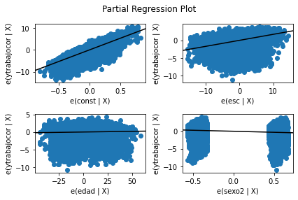
Por ejemplo, una visualización de las regresiones parciales se puede obtener mediante plot_partregress_grid. Esto muestra la relación entre la respuesta y la variable explicativa después de eliminar el efecto de todas las otras variables exógenas.
#Para ver gráficos de las regresiones parciales (regresionar la variable dependiente c/r a una variable condicional en el resto de las variables exógenas)
fig = sm.graphics.plot_partregress_grid(results)
fig.tight_layout(pad=1.0)
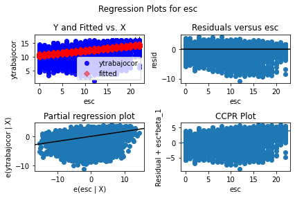
Para ver información de la regresión con respecto a una variable en específico podemos ocupar plot_regress_exog. Acá tenemos
Fitted plot
Residuo
Regresión parcial
Component-Component plus Residual (CCPR) plot: nos sirve para ver la relación entre uan variable independiente particular y la variable de respuesta, dado que otras variables indpendientes también están presentes en el modelo: \(Res+\hat{\beta}_iX_i\) versus \(X_i\)
fig = sm.graphics.plot_regress_exog(results, "esc")
fig.tight_layout(pad=1.0)
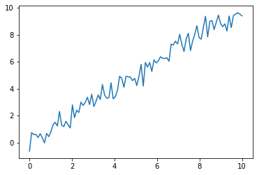
Ejemplo caso con menos ruido: ejemplo de juguete
x = np.linspace(0, 10, 100)
y = x + 0.5 * np.random.normal(size=len(x))

plt.plot(x,y)
[<matplotlib.lines.Line2D at 0x7f44946253d0>]
X = np.column_stack((x, x**2))
X = sm.add_constant(X)
res = sm.OLS(y, X).fit()
print(res.summary())
                            OLS Regression Results
==============================================================================
Dep. Variable:                      y   R-squared:                       0.974
Model:                            OLS   Adj. R-squared:                  0.973
Method:                 Least Squares   F-statistic:                     1807.
Date:                Mon, 26 Jul 2021   Prob (F-statistic):           1.73e-77
Time:                        23:31:42   Log-Likelihood:                -66.869
No. Observations:                 100   AIC:                             139.7
Df Residuals:                      97   BIC:                             147.6
Df Model:                           2
Covariance Type:            nonrobust
==============================================================================
                 coef    std err          t      P>|t|      [0.025      0.975]
------------------------------------------------------------------------------
const         -0.0904      0.141     -0.641      0.523      -0.370       0.189
x1             1.0865      0.065     16.670      0.000       0.957       1.216
x2            -0.0098      0.006     -1.557      0.123      -0.022       0.003
==============================================================================
Omnibus:                        0.781   Durbin-Watson:                   2.028
Prob(Omnibus):                  0.677   Jarque-Bera (JB):                0.817
Skew:                          -0.006   Prob(JB):                        0.665
Kurtosis:                       2.557   Cond. No.                         144.
==============================================================================

Notes:
[1] Standard Errors assume that the covariance matrix of the errors is correctly specified.
# y_hat = res.params[0] + results.params[1] * x + results.params[1] * x**2
res.params[2]
-0.009817635455210468
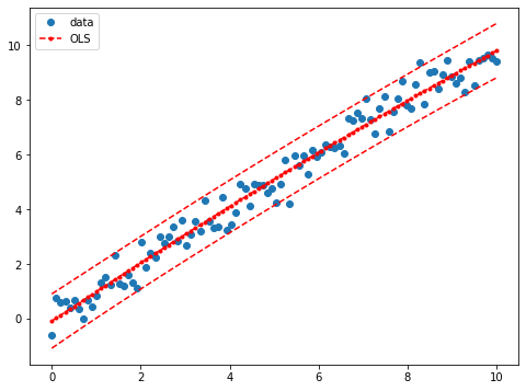
prstd, iv_l, iv_u = wls_prediction_std(res)
#Retorno:
#-standard error of prediction same length as rows of exog
#-lower und upper confidence bounds

fig, ax = plt.subplots(figsize=(8,6))

ax.plot(x, y, 'o', label="data")
ax.plot(x, res.fittedvalues, 'r--.', label="OLS")
ax.plot(x, iv_u, 'r--')
ax.plot(x, iv_l, 'r--')
ax.legend(loc='best');
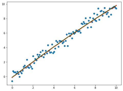
fig, ax = plt.subplots(figsize=(8,6))

y_hat = res.params[0] + res.params[1] * x + res.params[2] * x**2

ax.plot(x, y, 'o', label="data")
ax.plot(x, res.fittedvalues, 'r--.', label="OLS")
ax.plot(x, y_hat, 'g', label="OLS")
[<matplotlib.lines.Line2D at 0x7f4494171280>]
Modelo Autorregresivo (AR)
Podemos estimar un modelo del tipo \(Y_t = \beta_0 + \beta_1 Y_{t-1} + \mu_t\)
En python podemos utilizar AutoReg: https://www.statsmodels.org/stable/examples/notebooks/generated/autoregressions.html
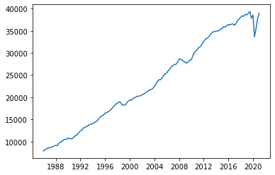
df = pd.read_excel("/home/felix/Dropbox/Computational_Economics/Intro_python/Data_OLS_AR/pib.xlsx")
df.dtypes
df.head()
| Periodo | PIB | |
|---|---|---|
| 0 | 1986-01-01 | 7899.666547 |
| 1 | 1986-04-01 | 8220.056395 |
| 2 | 1986-07-01 | 8355.276664 |
| 3 | 1986-10-01 | 8555.927503 |
| 4 | 1987-01-01 | 8626.993492 |
plt.plot(df.Periodo, df.PIB);
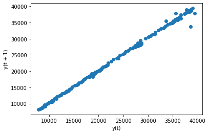
from pandas.plotting import lag_plot
lag_plot(df.PIB)
<AxesSubplot:xlabel='y(t)', ylabel='y(t + 1)'>
from statsmodels.tsa.ar_model import AutoReg, ar_select_order
from statsmodels.tsa.api import acf, pacf, graphics
mod = AutoReg(df.PIB, 1, old_names=False)
res = mod.fit()
print(res.summary())
                            AutoReg Model Results
==============================================================================
Dep. Variable:                    PIB   No. Observations:                  141
Model:                     AutoReg(1)   Log Likelihood               -1085.062
Method:               Conditional MLE   S.D. of innovations            562.000
Date:                Tue, 27 Jul 2021   AIC                             12.706
Time:                        08:19:50   BIC                             12.769
Sample:                             1   HQIC                            12.731
                                  141
==============================================================================
                 coef    std err          z      P>|z|      [0.025      0.975]
------------------------------------------------------------------------------
const        257.5324    123.602      2.084      0.037      15.278     499.787
PIB.L1         0.9985      0.005    203.603      0.000       0.989       1.008
                                    Roots
=============================================================================
                  Real          Imaginary           Modulus         Frequency
-----------------------------------------------------------------------------
AR.1            1.0015           +0.0000j            1.0015            0.0000
-----------------------------------------------------------------------------
Podemos actualizar el modelo a \(Y_t = \beta_0 + \beta_1 Y_{t-1} + \beta_2 Y_{t-2} + \beta_3 Y_{t-3} + \beta_4 Y_{t-4} + \beta_5 Y_{t-5} + \mu_t\)
mod = AutoReg(df.PIB, 5, old_names=False)
res = mod.fit()
print(res.summary())
                            AutoReg Model Results
==============================================================================
Dep. Variable:                    PIB   No. Observations:                  141
Model:                     AutoReg(5)   Log Likelihood               -1047.475
Method:               Conditional MLE   S.D. of innovations            535.438
Date:                Tue, 27 Jul 2021   AIC                             12.669
Time:                        08:21:12   BIC                             12.819
Sample:                             5   HQIC                            12.730
                                  141
==============================================================================
                 coef    std err          z      P>|z|      [0.025      0.975]
------------------------------------------------------------------------------
const        423.0718    133.111      3.178      0.001     162.179     683.965
PIB.L1         0.8942      0.083     10.802      0.000       0.732       1.056
PIB.L2         0.2591      0.123      2.105      0.035       0.018       0.500
PIB.L3        -0.3180      0.120     -2.658      0.008      -0.553      -0.083
PIB.L4        -0.5179      0.223     -2.323      0.020      -0.955      -0.081
PIB.L5         0.6816      0.195      3.488      0.000       0.299       1.065
                                    Roots
=============================================================================
                  Real          Imaginary           Modulus         Frequency
-----------------------------------------------------------------------------
AR.1           -0.8762           -0.6971j            1.1197           -0.3930
AR.2           -0.8762           +0.6971j            1.1197            0.3930
AR.3            0.7558           -0.7735j            1.0814           -0.1268
AR.4            0.7558           +0.7735j            1.0814            0.1268
AR.5            1.0006           -0.0000j            1.0006           -0.0000
-----------------------------------------------------------------------------
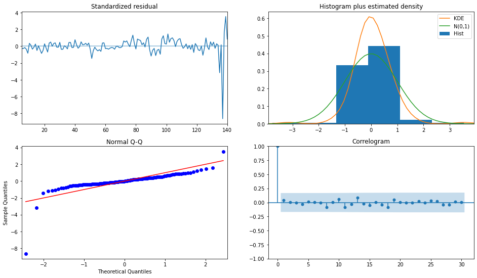
Para un resumen de la visualización de los residuos estandarizados podemos ocupar plot_diagnostics
fig = plt.figure(figsize=(16,9))
fig = res.plot_diagnostics(fig=fig, lags=30)
#Standarized residual:
    #-residuo: Valor observado - valor predicho
    #-standarized residual: residuo normalizado por el error estandar del modelo (RSE)
#Histogram plus: estima la distribución de los residuos estandarizados. Nos muestra la distribución normal (línea verde) como punto de comparación.
#Normal Q-Q : muestra si el residuo está distribuido normalmente. Lo que se espera es que los puntos se encuentren sobre la línea roja o cercanos a ella.
#Correlograma: nos muestra un gráfico de autocorrelaciones
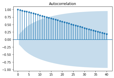
Autocorrelaciones: https://www.statsmodels.org/stable/generated/statsmodels.graphics.tsaplots.plot_acf.html
sm.graphics.tsa.plot_acf(df.PIB, lags=40)
plt.show()
Actividad
Estime la ecuación de mincer: \(Ingreso_i = \beta_0 + \beta_1 esc_i + \beta_2 exp_i + \beta_3 exp_i^2 + \beta_4 sexo_i + \mu_i\) donde :
ingreso: log(ingreso del trabajo)
esc: escolaridad
exp: experiencia = edad - escolaridad
exp2: expediencia al cuadrado
sexo: variable dicotómica si es hombre (0) o mujer (1).
Estime un modelo AR del tipo \(\Delta y_t = \Delta y_{t-1}\) donde:
\(y_t\) es el PIB trimestral en el periodo t.
\(\Delta y_t\) es la variación del PIB trimestral en el periodo t.
\(\Delta y_{t-1}\) es la variación del PIB trimestral en el periodo t-1.